House Price Prediction

🏡 House Price Prediction Using Linear Regression

MAIN TOOL

R Programming Language

Technique

Linear Regression Analysis

INDUSTRY

Housing

📚 About the Project

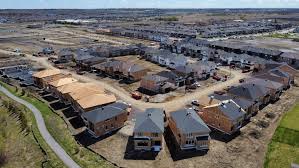
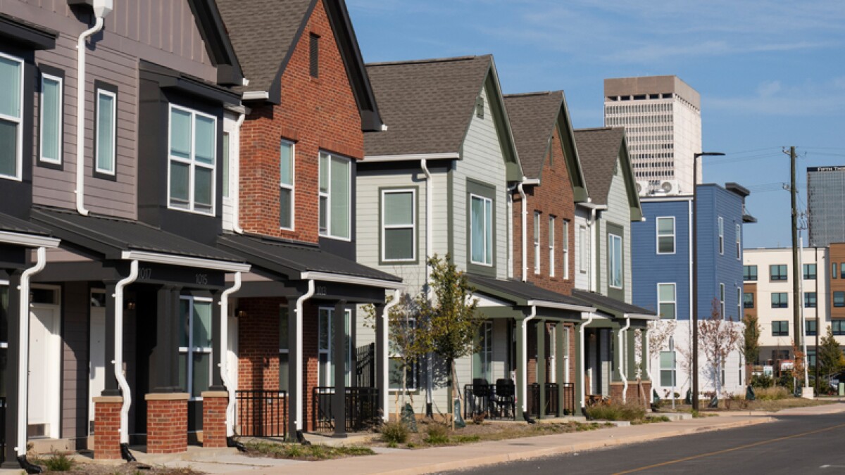
This project leverages Linear Regression to predict house prices based on the Ames Housing Dataset, which provides detailed information on housing sales in Ames, Iowa. The analysis focuses on identifying significant predictors of house prices and refining the regression model to improve predictive accuracy.

🔑 Key Features

Data Preprocessing:
- Addressed missing values using advanced imputation techniques like MICE.
- Focused on key continuous variables such as Gr.Liv.Area, Total.Bsmt.SF, Garage.Area, etc.
- Handled outliers through visual diagnostics and statistical tests.
Regression Modeling:
- Built and refined multiple linear regression models.
- Included interaction terms and performed all subsets regression for model selection.
- Addressed multicollinearity using Variance Inflation Factors (VIF).
Model Evaluation:
- Evaluated models using Adjusted R-Squared, AIC, BIC, and F-statistics.
- Diagnostic plots such as Residuals vs. Fitted, Scale-Location, and Q-Q Plots.
Business Impact:
- Insights into factors influencing house prices, aiding real estate professionals in pricing strategies.

📊 Key Insights

Significant Predictors:
- Gr.Liv.Area (Above Ground Living Area): The strongest positive predictor of house price.
- Total.Bsmt.SF (Basement Area): A significant contributor to house value.
- Garage.Area: Highly valued by buyers, as reflected in its positive coefficient.
Best Model:
- A three-variable interaction model with the highest Adjusted R-Squared (76.73%).
- Equation: [ SalePrice = 69,940 + 0.0628 \times (Gr.Liv.Area \times Garage.Area) + 0.1515 \times (Garage.Area \times Total.Bsmt.SF) + 0.3489 \times (Gr.Liv.Area \times Total.Bsmt.SF) ]
Model Comparison:
- The interaction model outperformed simpler models with lower AIC/BIC scores and better predictive power.

📜 Full Report

For a detailed analysis, including methodology, visualizations, and results, refer to the complete project report:
📄 House Price Prediction Report

📂 Project Structure

.
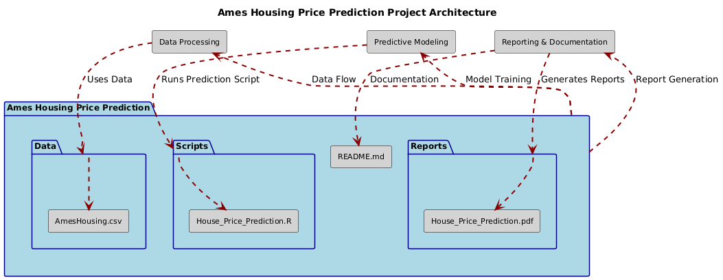
├── Data/
│   ├── AmesHousing.csv
├── Scripts/
│   ├── House_Price_Prediction.R
├── Reports/
│   ├── House_Price_Prediction.pdf
├── README.md

🤝 Connect with Me

Feel free to reach out for feedback, questions, or collaboration opportunities:
LinkedIn: Dr. Syed Faizan

Author: Syed Faizan
Master’s Student in Data Analytics and Machine Learning

Github Repository

R Code and the Report of the Analysis

	#---------------------------------------------------------#
	# Syed Faizan #
	# House Price Prediction #
	# #
	# #
	# #
	# #
	#---------------------------------------------------------#

	#Starting with a clean environment

	rm(list=ls())


	# Clearing the Console
	cat("\014")

	#Loading the packages utilized for Data cleaning and Data Analysis

	library(tidyverse)
	library(grid)
	library(gridExtra)
	library(dplyr)
	library(ggplot2)


	# Loading the Data set

	ames <- read.csv("AmesHousing.csv")


	# Performing Exploratory Data Analysis and using descriptive statistics to describe the data.

	head(ames)
	summary(ames) # To note: Total basement Area has minimum of zero, showing no basement in some houses

	# Get the data types that constitute this data set using a function
	variable_types <- function(x) {
	sapply(x, class)
	}
	variable_types(ames)

	# We find the number of numeric variables

	numeric_variables <- function(x) {
	num_vars <- sum(sapply(x, is.numeric))
	return(num_vars)
	}

	numeric_variables <- numeric_variables(ames)
	print(paste("Number of numeric variables:", numeric_variables))

	# We find the number of categorical variables
	count_categorical_variables <- function(x) {
	cat_vars <- sum(sapply(x, is.factor)) + sum(sapply(x, is.character))
	return(cat_vars)
	}

	categorical_variable_count <- count_categorical_variables(ames)
	print(paste("Number of categorical variables:", categorical_variable_count))


	# We create a new column called age from the year built column
	max(ames$Year.Built)

	ames$Age <- max(ames$Year.Built) - ames$Year.Built

	# Check the head of the dataset to verify the new column
	head(ames)
	# Check the maximum and minimum of 'age'

	min(ames$Age)
	max(ames$Age)

	# We check for n/a values among the variables
	library(dlookr)

	plot_na_hclust(ames)

	# We create a function to verify the missing values in the most affected columns

	miss_sum <- function(x) {

	print(sum(is.na(x)))}

	c <- c(ames$Pool.QC, ames$Misc.Feature, ames$Alley, ames$Fence, ames$Fireplace.Qu)

	miss_sum(c)

	# We discard these columns from the Dataset
	ames$Pool.QC <- NULL
	ames$Misc.Feature <- NULL
	ames$Alley <- NULL
	ames$Fence <- NULL
	ames$Fireplace.Qu <- NULL

	# Lookng for proportion of missing values left

	plot_na_pareto(ames, only_na = TRUE)





	# In fulfillment of question number 3 of the assignment we impute values to the numeric
	# variables that have missing values and are of relevance to further analysis

	sum(is.na(ames$Total.Bsmt.SF))
	sum(is.na(ames$Mas.Vnr.Area))
	sum(is.na(ames$Lot.Frontage))


	# Since Lot Frontage has 490 missing values we shall use machine learning
	# to impute missing values so as to not alter the distribution

	library(ranger)



	imputate_na(ames, Lot.Frontage, Lot.Area , method = 'mean' ) %>%
	plot()

	imputate_na(ames, Lot.Frontage, Lot.Area , method = 'mice' ) %>%
	plot()


	library(mice)

	imputed_data <- mice(ames[, c("Lot.Frontage", "Lot.Area")], m = 5, seed = 123, method = 'pmm')

	completed_data <- complete(imputed_data, 1)

	ames$Lot.Frontage <- completed_data$Lot.Frontage
	ames$Lot.Area <- completed_data$Lot.Area

	# checking proper imputation
	sum(is.na(ames$Lot.Frontage))
	# Since the other two relevant columns have only 1 value and 23 values missing
	# we shall impute missing values using the mean

	mean_Total_Bsmt_SF <- mean(ames$Total.Bsmt.SF, na.rm = TRUE)

	ames$Total.Bsmt.SF[is.na(ames$Total.Bsmt.SF)] <- mean_Total_Bsmt_SF


	mean_Mas_Vnr_Area <- mean(ames$Mas.Vnr.Area, na.rm = TRUE)

	ames$Mas.Vnr.Area[is.na(ames$Mas.Vnr.Area)] <- mean_Mas_Vnr_Area



	#checking proper imputation


	sum(is.na(ames$Total.Bsmt.SF))
	sum(is.na(ames$Mas.Vnr.Area))

	# As the number of numeric variables is 39, which is large
	# We use domain knowledge to focus on a smaller number of numeric variables that are relevant
	# so as to visualize them in a 5 number summary table

	# Creating a numeric-variable-only data set.

	amesn <- ames %>%
	select(Gr.Liv.Area, Total.Bsmt.SF, Garage.Area, Lot.Frontage, Lot.Area, SalePrice, Age)

	# Creating descriptive statistics table

	library(dlookr)

	descriptive_table <- amesn %>%
	diagnose_numeric()

	library(DT)

	# Creating an interactive table available as Webpage at https://rpubs.com/SyedFaizan2024/1173195

	datatable(descriptive_table, options = list(pageLength = 5), caption = "Descriptive Statistics of the Ames Housing Dataset")


	# Visualizing the Numeric Variables


	library(DataExplorer)
	plot_histogram(amesn)

	plot_density(amesn)


	# Visualizing outliers
	plot_outlier(amesn)

	# Checking for normality of distribution of the numeric variables

	plot_normality(amesn)

	# Feature engineering

	# We notice that adding a logarithmic transformation of the response variable
	# Saleprice might improve our putative model
	ames$LogSalePrice <- log(ames$SalePrice)
	amesn$LogSalePrice <- log(ames$SalePrice)

	# We also add masonry veneer area and enclosed porch area to the numerical variable dataset
	amesn <- amesn %>% mutate(Mas.Vnr.Area = ames$Mas.Vnr.Area)
	amesn <- amesn %>% mutate(Enclosed.Porch = ames$Enclosed.Porch)

	# Checking if outliers need to be removed by examining scatter plots between
	# numerical variables
	library(GGally)

	ggpairs(amesn) +
	ggtitle("Pairwise relationships in amesn dataset") +
	xlab("Variables on X-axis") +
	ylab("Variables on Y-axis")

	# Noticing Outliers in the important relationship between Living Area above ground
	# and Sale Price
	# plot Sale price against Living Area above ground

	plot( ames$Gr.Liv.Area, ames$SalePrice )

	# investigating the outliers in terms of neighborhood

	ames %>% filter( Gr.Liv.Area > 4000 ) %>% arrange( SalePrice )

	# Is the neighborhood the reason why these outliers are so huge?
	ames %>% group_by( Neighborhood ) %>%
	summarize( size = mean( Gr.Liv.Area ) ) %>%
	print( n = Inf )

	# Mean Gr.Liv.Area in Edwards is 1338 so neighborhood does not explain variation


	# finding the outlier indices
	outliers <- ames$Gr.Liv.Area > 4000 & ames$SalePrice < 300000
	ames[outliers,]

	# fit simple linear regression models to determine leverage
	m1 <- lm( SalePrice ~ Gr.Liv.Area, data = ames )
	m2 <- lm( SalePrice ~ Gr.Liv.Area, data = ames, subset = !outliers )


	# Visualize the influence of the variables
	plot( ames$Gr.Liv.Area, ames$SalePrice )
	abline(m1, col = "blue")
	abline(m2, col = "green")

	# We decide to remove three outliers after careful consideration

	# Creating a new dataset 'amesclean' by excluding these outliers

	amesclean <- ames[!outliers, ]

	#remove the one missing value from 'amesclean' by imputing mean

	# Calculating the mean of Garage.Area excluding NA values
	mean_Garage_Area <- mean(amesclean$Garage.Area, na.rm = TRUE)

	# Replacing NA values in Garage.Area with the computed mean
	amesclean$Garage.Area[is.na(amesclean$Garage.Area)] <- mean_Garage_Area


	# Incorporate desired numerical variables into a new numeric dataset
	# from 'amesclean' for correlation analysis

	amesn3 <- amesclean %>% select(where(is.numeric))



	# Checking the correlation between different numerical variables

	cor(amesn3, use = 'complete.obs')
	cor_matrix <- cor(amesn3, use = 'complete.obs')



	library(ggcorrplot)
	ggcorrplot(
	cor_matrix,
	hc.order = TRUE, # Reorders the matrix using hierarchical clustering
	lab = TRUE, # Set to FALSE if too cluttered
	sig.level = 0.05,
	insig = "blank", # Leaves insignificant correlations blank
	lab_size = 2.5, # Adjust text size; may need to lower if too cluttered
	title = "Correlation matrix for the Ames Housing Dataset"
	)


	# scatter plot for the X continuous variable with the highest correlation with SalePrice
	plot(
	amesclean$SalePrice,
	amesclean$Gr.Liv.Area,
	main = 'Scatter plot for the Above Grade Living Area and Sale Price',
	xlab = "Sale Price",
	ylab = "Above Grade Living Area (sq ft)",
	col = rainbow(length(amesclean$SalePrice)), # Rainbow colors for each point
	pch = 19 # Solid circle
	)

	# scatter plot for the X variable that has the lowest correlation with SalePrice
	plot(
	amesclean$SalePrice,
	amesclean$BsmtFin.SF.2,
	main = 'Scatterplot for Type 2 Basement Finished Area and Sale Price',
	xlab = "Sale Price",
	ylab = "Type 2 Basement Finished Area (sq ft)",
	col = "darkgreen",
	pch = 19 # Solid circle
	)

	# scatter plot between X and SalePrice with the correlation closest to 0.5

	plot(
	amesclean$SalePrice,
	amesclean$Mas.Vnr.Area,
	main = 'Scatterplot for Masonry Veneer Area and Sale Price',
	xlab = "Sale Price",
	ylab = "Masonry Veneer Area (sq ft)",
	col = "orange",
	pch = 19
	)

	model <- lm(SalePrice ~ Gr.Liv.Area + Total.Bsmt.SF + X1st.Flr.SF + Garage.Area, data = amesclean)


	# each coefficient of the model in the context of this problem.

	summary(model)
	coefficients(model)

	# Interpret the four graphs that are produced.
	plot(model)

	library(car)
	vif_values <- vif(model)
	print(vif_values)



	# Performing outlier test on the model
	outlier_test <- outlierTest(model)

	# Displaying the results of the outlier test
	print(outlier_test)

	# Function to plot the hat values (leverages)
	hat.plot <- function(model) {
	p <- length(coefficients(model)) # number of model parameters
	n <- length(fitted(model)) # number of observations
	plot(hatvalues(model), main ="Index Plot of Hat Values")
	abline(h= 2 * p/n, col = "orange", lty = 2) # cutoff line for potential high leverage points
	identify(1:n, hatvalues(model), names(hatvalues(model)))
	}
	hat.plot(model) # Calling the function with the linear model

	# Identifying influential observations based on Cook's distance
	cooksd <- cooks.distance(model)
	cutoff <- 4 / nrow(amesclean) # Common rule of thumb for Cook's distance cutoff

	# Creating a plot to visualize Cook's distance for each observation
	plot(cooksd, pch = 19, main = "Cook's Distance Cutoff Plot",
	xlab = "Observation Index", ylab = "Cook's Distance")
	abline(h = cutoff, col = "red", lty = 2) # Line representing the cutoff value

	# Highlighting influential observations that exceed the cutoff
	influential_obs <- which(cooksd > cutoff)
	points(influential_obs, cooksd[influential_obs], col = "red", pch = 19)

	# Question 12 Attempt to correct any issues that you have discovered in your model.
	# Did your changes improve the model, why or why not?

	# In order to refine my model I need to closely inspect the outliers

	order_numbers <- c(45, 1768, 1064, 1761, 2593, 433, 434, 2446, 2333, 2335)

	# Using filter() to extract rows which are the outliers
	rows_to_inspect <- amesclean %>%
	filter(Order %in% order_numbers)

	# Print the rows to get a better idea of the data
	print(rows_to_inspect)

	# Seven out of ten outliers are from the same two neighborhoods suggesting a pattern
	# I decided to remove only the abnormal sale condition outlier in row 1761
	# and the house in row 2593 because its age was very high i.e it was oddly old
	rows_to_remove <- c(1761, 2593)

	# Creating a new dataset without the specified outliers
	amesclean2 <- amesclean %>%
	filter(!Order %in% rows_to_remove)

	# I have also decided to drop 'X1st.Flr.SF' that is the first floor square feet
	# due to its high p value in the earlier model

	model_updated <- lm(SalePrice ~ Gr.Liv.Area + Total.Bsmt.SF + Garage.Area, data = amesclean2)

	# Checking the summary of the updated model
	summary(model_updated)

	# plotting the new model
	plot(model_updated)

	# Question 13 . Use the all subsets regression method to identify the "best" model. State the preferred model in equation form.

	library(leaps)

	# Running the regsubsets function with interaction and squared terms

	best_subsets <- regsubsets(SalePrice ~ (Gr.Liv.Area + Total.Bsmt.SF + Garage.Area)^2,
	data = amesclean2, nvmax = 3, method = "exhaustive")

	# Extracting the summary of the best subsets, focusing on adjusted R-squared
	print(best_subsets)

	subsets_summary <- summary(best_subsets)

	subsets_summary$adjr2 # subsets_summary$adjr2
	# [1] 0.6859263 0.7659139 0.7673065
	subsets_summary$bic
	#Visualizing the models
	library(car)

	subsets(best_subsets, statistic = "adjr2", ylim = c(0.67,0.77))


	#Implementing the best subset regression model based on three predictors
	best_model <- lm(SalePrice ~ Gr.Liv.Area: Garage.Area + Total.Bsmt.SF: Garage.Area + Gr.Liv.Area:Total.Bsmt.SF,data = amesclean2)

	summary(best_model)



	#comparing the two models

	summary_best_model <- summary(best_model)
	summary_model_updated <- summary(model_updated)

	# Creating a data frame to compare vital metrics
	comparison <- data.frame(
	Model = c("best_model", "model_updated"),
	Adjusted_Rsquared = c(summary_best_model$adj.r.squared, summary_model_updated$adj.r.squared),
	AIC = c(AIC(best_model), AIC(model_updated)),
	BIC = c(BIC(best_model), BIC(model_updated)),
	Fstatistic = c(summary_best_model$fstatistic[1], summary_model_updated$fstatistic[1]),
	Residual_SE = c(summary_best_model$sigma, summary_model_updated$sigma)
	)

	#The comparison
	print(comparison)

	# The end of the project

view raw HousePrice.R hosted with ❤ by GitHub