Heart Disease Diagnosis

❤️ Heart Disease Prediction Using Support Vector Machines (SVM)

MAIN TOOL

R Programming Language

Technique

Support Vector Machines

INDUSTRY

Medicine

📚 About the Project

This project applies Support Vector Machines (SVM) to the Heart Disease dataset for the classification of patients into two categories: “No Disease” and “Disease.” The goal is to develop a robust predictive model that can assist healthcare professionals in identifying heart disease cases based on clinical and demographic variables.

🔑 Key Features:

Data Preprocessing:
- Comprehensive data cleaning, feature engineering, and scaling for effective SVM implementation.
Classification Models:
- Developed models using linear and radial kernels.
Hyperparameter Tuning:
- Optimized SVM parameters using grid search and cross-validation for better classification accuracy.
Performance Evaluation:
- Evaluated models using accuracy, sensitivity, specificity, precision, and ROC curves.

📊 Key Insights

Best Model: The tuned SVM with a radial kernel achieved:
- Accuracy: 99.03%
- Sensitivity (Recall): 100%
- Specificity: 97.93%
- Precision: 98.19%
Clinical Impact:
- High sensitivity ensures no cases of heart disease are missed.
- Robust predictions make the model suitable for deployment in medical diagnostics.

🖥️ Live Application

For a detailed walkthrough of the analysis, refer to the complete project report:
📄 Heart Disease Diagnosis Report

📂 Project Structure

.
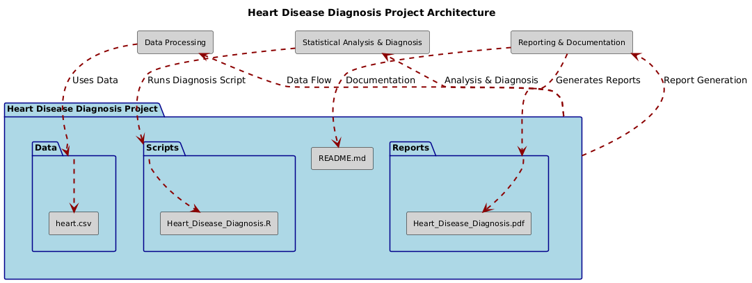
├── Data/
│   ├── heart.csv
├── Scripts/
│   ├── Heart_Disease_Diagnosis.R
├── Reports/
│   ├── Heart_Disease_Diagnosis.pdf
├── README.md

🤝 Connect with Me

Feel free to reach out for feedback, questions, or collaboration opportunities:
LinkedIn: Dr. Syed Faizan

Author: Syed Faizan
Master’s Student in Data Analytics and Machine Learning

Github Repository

R Code and the Report of the Analysis

	#---------------------------------------------------------#
	# Syed Faizan #
	# Heart Disease Diagnosis using SVM's #
	# #
	# #
	# #
	# #
	#---------------------------------------------------------#

	#Starting with a clean environment----

	rm(list=ls())


	# Clearing the Console
	cat("\014") # Clears the console

	# Clearing scientific notation

	options(scipen = 999)

	#Loading the packages utilized for Data cleaning and Data Analysis-----



	library(tidyverse)
	library(grid)
	library(gridExtra)
	library(dplyr)
	library(kableExtra)
	library(ggplot2)
	library(DataExplorer)
	library(dlookr)
	library(lubridate)
	library(table1)
	library(psych)

	# Loading the initial Data set
	heartdf <- read.csv('heart.csv')

	str(heartdf) # confirming structure of the data set

	summary(heartdf)

	head(heartdf)
	tail(heartdf)


	any(is.na(heartdf)) # Analyzing and visualizing the missing data

	sum(is.na(heartdf))

	plot_missing(heartdf)


	# Feature Engineering
	# Data transformation of target variable to factor

	heartdf$target <- factor(heartdf$target, labels = c("NoDisease", "Disease"))

	# Defining the label for each variable for clarity in the table
	label(heartdf$age) <- "Age"
	label(heartdf$sex) <- "Sex"
	label(heartdf$cp) <- "Chest Pain Type (CP)"
	label(heartdf$trestbps) <- "Resting Blood Pressure (trestbps)"
	label(heartdf$chol) <- "Cholesterol (chol)"
	label(heartdf$fbs) <- "Fasting Blood Sugar (fbs)"
	label(heartdf$restecg) <- "Resting ECG (restecg)"
	label(heartdf$thalach) <- "Maximum Heart Rate Achieved (thalach)"
	label(heartdf$exang) <- "Exercise-Induced Angina (exang)"
	label(heartdf$oldpeak) <- "ST Depression (oldpeak)"
	label(heartdf$slope) <- "Slope of ST Segment (slope)"
	label(heartdf$ca) <- "Number of Major Vessels (ca)"
	label(heartdf$thal) <- "Thalassemia (thal)"

	# Convert 'sex' to a factor with appropriate labels
	heartdf$sex <- factor(heartdf$sex, levels = c(0, 1), labels = c("Female", "Male"))

	# Convert 'cp' (chest pain type) to a factor with appropriate labels
	heartdf$cp <- factor(heartdf$cp, levels = c(0, 1, 2, 3),
	labels = c("Typical Angina", "Atypical Angina", "Non-Anginal Pain", "Asymptomatic"))

	# Convert 'fbs' (fasting blood sugar > 120 mg/dl) to a factor with appropriate labels
	heartdf$fbs <- factor(heartdf$fbs, levels = c(0, 1), labels = c("False", "True"))

	# Convert 'restecg' to a factor with appropriate labels
	heartdf$restecg <- factor(heartdf$restecg, levels = c(0, 1, 2),
	labels = c("Normal", "ST-T Wave Abnormality",
	"Left Ventricular Hypertrophy"))

	# Convert 'exang' (exercise-induced angina) to a factor with appropriate labels
	heartdf$exang <- factor(heartdf$exang, levels = c(0, 1), labels = c("No", "Yes"))

	# Convert 'slope' to a factor with appropriate labels
	heartdf$slope <- factor(heartdf$slope, levels = c(0, 1, 2),
	labels = c("Upsloping", "Flat", "Downsloping"))

	# Convert 'thal' to a factor with appropriate labels
	heartdf$thal <- factor(heartdf$thal, levels = c(0, 1, 2, 3),
	labels = c("Unknown", "Normal", "Fixed Defect", "Reversible Defect"))



	# Create table1 stratified by the target variable
	# Load necessary library
	library(table1)

	# Categorical variables
	table1(~ sex + cp + fbs + restecg + exang + slope + thal \| target,
	data = heartdf)

	# Numerical variables
	table1(~ age + trestbps + chol + thalach + oldpeak + ca \| target,
	data = heartdf)

	# Data Visualization
	# Create a data frame for categorical variables
	cat_df <- heartdf[, c("sex", "cp", "fbs", "restecg", "exang", "slope", "thal", "target")]

	# Create a data frame for numerical variables
	num_df <- heartdf[, c("age", "trestbps", "chol", "thalach", "oldpeak", "ca")]

	# Check the structure of the new data frames
	str(cat_df)
	str(num_df)

	# Checking if the numerical variables need scaling
	means <- sapply(num_df[, -7], mean)
	stddevs <- sapply(num_df[, -7], sd)

	scaling_check <- cbind(means, stddevs)
	print(scaling_check)

	# Scaling is needed, however it shall be done after visualization

	library(dlookr)
	library(DataExplorer)

	plot_outlier(num_df, col = "red")

	plot_normality(num_df, col = "yellow")

	plot_bar_category(cat_df)

	# Correlation Matrix
	library(ggcorrplot)
	ggcorrplot(cor(num_df), lab = TRUE)

	# Pair Plots
	library(GGally)
	ggpairs(num_df)


	# Scaling
	# Ensure the 'target' column is not scaled and is retained as is
	num_df <- num_df[, 1:6] # Extract the target column

	# Scale the remaining numerical columns (exclude 'target' column)
	num_df_scaled <- scale(num_df, center = TRUE, scale = TRUE)

	# Combine the scaled data with the 'target' column
	num_df <- data.frame(num_df_scaled)

	# Ensure 'target' is a factor in num_df
	# Convert 'target' in num_df to a factor with levels "NoDisease" and "Disease"
	num_df$target <- factor(heartdf$target)


	# Divide into test and train
	# Set seed for reproducibility
	set.seed(314)

	# Split the data into 70% training and 30% testing
	train_index <- sample(1:nrow(num_df_scaled), size = 0.7 * nrow(num_df_scaled))

	# Create training and testing datasets
	train_data <- num_df[train_index, ]
	test_data <- num_df[-train_index, ]

	# Check dimensions of the train and test sets
	dim(train_data) # Should be 70% of the total rows
	dim(test_data) # Should be 30% of the total rows

	# SVM Implementation

	library(e1071)
	library(caret)

	# Train an SVM model with linear kernel on the training data
	svmfit <- svm(target ~ ., data = train_data, kernel = "linear", cost = 10, scale = FALSE)
	summary(svmfit)

	# Predictions on test data
	ypred <- predict(svmfit, newdata = test_data)

	# Confusion matrix using confusionMatrix from caret
	conf_matrix <- confusionMatrix(ypred, test_data$target)
	print(conf_matrix)

	# Tune SVM model to find best cost parameter
	set.seed(1)
	tune.out <- tune(svm, target ~ ., data = train_data, kernel = "linear",
	ranges = list(cost = c(0.001, 0.01, 0.1, 1, 10, 100)))
	summary(tune.out)

	# Use the best model found through tuning
	bestmod <- tune.out$best.model
	summary(bestmod)

	# Predictions using the best model on test data
	ypred_best <- predict(bestmod, newdata = test_data)

	# Confusion matrix for the best tuned model
	conf_matrix_best <- confusionMatrix(ypred_best, test_data$target)
	print(conf_matrix_best)

	# Support Vector Machine with Radial Kernel
	svmfit_radial <- svm(target ~ ., data = train_data, kernel = "radial", gamma = 1, cost = 1)
	summary(svmfit_radial)

	# Predictions using Radial Kernel SVM
	ypred_radial <- predict(svmfit_radial, newdata = test_data)

	# Confusion matrix for Radial Kernel
	conf_matrix_radial <- confusionMatrix(ypred_radial, test_data$target)
	print(conf_matrix_radial)

	# Tune SVM with Radial Kernel to find the best cost and gamma parameters
	set.seed(144)
	tune.out_radial <- tune(svm, target ~ ., data = train_data, kernel = "radial",
	ranges = list(cost = c(0.1, 1, 10, 100, 1000), gamma = c(0.5, 1, 2, 3, 4)))
	summary(tune.out_radial)

	# Use the best radial model found through tuning
	bestmod_radial <- tune.out_radial$best.model

	# Predictions using the best radial model
	ypred_best_radial <- predict(bestmod_radial, newdata = test_data)

	# Confusion matrix for the best radial model
	conf_matrix_best_radial <- confusionMatrix(ypred_best_radial, test_data$target)
	print(conf_matrix_best_radial)

	# ROC Curve for the Radial SVM Model
	library(ROCR)

	rocplot <- function(pred, truth, ...) {
	predob <- prediction(pred, truth)
	perf <- performance(predob, "tpr", "fpr")
	plot(perf, ...)
	}

	# Obtain decision values for plotting ROC
	svmfit_opt <- svm(target ~ ., data = train_data, kernel = "radial", gamma = 2, cost = 1, decision.values = TRUE)
	fitted <- attributes(predict(svmfit_opt, train_data, decision.values = TRUE))$decision.values

	# Plot ROC Curve for training data
	par(mfrow = c(1, 2))
	rocplot(fitted, train_data$target, main = "Training Data (Radial Kernel)")

	# Obtain decision values for the test set
	fitted_test <- attributes(predict(svmfit_opt, test_data, decision.values = TRUE))$decision.values

	# Plot ROC Curve for test data
	rocplot(fitted_test, test_data$target, main = "Test Data (Radial Kernel)")

	# The Project Ends

view raw HeartDisease.R hosted with ❤ by GitHub