College Graduation Rate Prediction

🎓 College Graduation Rate Prediction Using Ridge and LASSO Regression

MAIN TOOL

R Programming Language

Technique

Linear Regression with Regularization

INDUSTRY

Education

📚 About the Project

This project employs Ridge and LASSO Regression to predict college graduation rates based on a rich dataset of U.S. colleges. The project uses the College dataset from the ISLR package, which contains information about U.S. colleges and universities, including tuition fees, student demographics, and graduation rates.

By utilizing regularization techniques, this project addresses issues of multicollinearity, selects significant predictors, and provides actionable insights for improving educational outcomes.

🔑 Key Features

Data Preprocessing:
- Comprehensive exploration and cleaning of the dataset.
- Analysis of multicollinearity and feature engineering.
Modeling Techniques:
- Ridge Regression (L2 Regularization).
- LASSO Regression (L1 Regularization).
- Stepwise Regression for model comparison.
Model Evaluation:
- Comparison of RMSE for Ridge, LASSO, and Stepwise Regression.
- Validation of overfitting and generalization using training and testing datasets.
Visualization:
- Detailed plots showing regularization paths, deviance explained, and variable importance.

📊 Key Insights

Best Model: Ridge Regression outperformed other models with the lowest RMSE.
Significant Predictors:
- Private: Private colleges have higher graduation rates compared to public institutions.
- Top10perc and Top25perc: A higher proportion of top-performing students positively impacts graduation rates.
- perc.alumni: Alumni engagement strongly correlates with higher graduation rates.
Overfitting:
- Ridge and LASSO models showed minimal overfitting, ensuring robustness.

📜 Full Report

For a detailed analysis, including methodology, regularization plots, and insights, refer to the complete project report:
📄 College Graduation Rate Prediction Report

📂 Project Structure

.
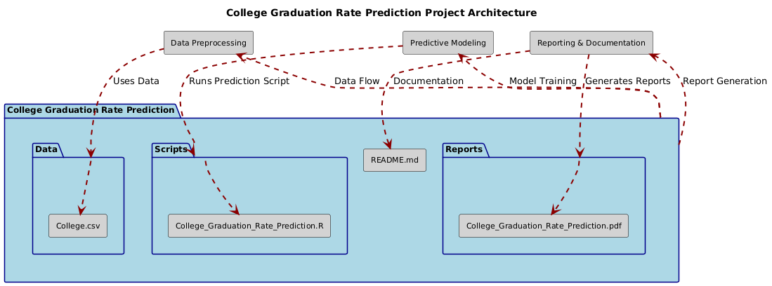
├── Data/
│   ├── College.csv
├── Scripts/
│   ├── College_Graduation_Rate_Prediction.R
├── Reports/
│   ├── College_Graduation_Rate_Prediction.pdf
├── README.md

🤝 Connect with Me

Feel free to reach out for feedback, questions, or collaboration opportunities:
LinkedIn: Dr. Syed Faizan

Author: Syed Faizan
Master’s Student in Data Analytics and Machine Learning

Github Repository

R Code and the Report of the Analysis

	#---------------------------------------------------------#
	# Syed Faizan #
	# College Graduation Rate Prediction #
	# #
	# #
	# #
	# #
	#---------------------------------------------------------#

	# Starting with a clean environment

	rm(list=ls())


	# Clearing the Console
	cat("\014") # Clears the console

	# Removing Scientific Notation
	options(scipen = 999)

	# Loading the packages utilized for Data cleaning and Data Analysis



	library(tidyverse)
	library(grid)
	library(gridExtra)
	library(dplyr)
	library(ggplot2)
	library(ISLR)
	library(caret)
	library(vtable)
	library(dlookr)
	library(DataExplorer)
	library(psych)
	library(pROC)
	library(ggcorrplot)
	library(glmnet)


	# Loading the College Dataset

	College <- College

	dim(cl)
	names(cl)
	summary(cl)
	View(cl)
	class(cl)


	# Since Graduation Rate is the response variable prescribed in our assignment
	# I wish to take a closer look at it through box plots




	ggplot(cl, aes(x = Private, y = Grad.Rate, fill = Private)) +
	geom_boxplot( alpha = 0.7, col = c("red", "blue")) +
	labs(title = "Graduation Rate by College Type",

	y = "Graduation Rate (%)",
	fill = "Is the College Private?") +
	theme(legend.position = "bottom",
	plot.title = element_text(hjust = 0.5), # Center the title
	legend.title.align = 0.5) + # Center the legend title
	ylim(0, 120) # Limit Y-axis to valid graduation rates

	# Descriptive Statistics Table for the Dataset

	st(cl)


	# RIDGE
	# Assignment Question 1

	# Split the data into a train and test set – refer to the Feature_Selection_R.pdf
	# document for information on how to split a dataset.

	# Partition data indices for a 70% training set
	set.seed(123) # for reproducibility
	trainIndex <- createDataPartition(y = College$Private, p = 0.7, list = FALSE)
	train <- College[trainIndex, ]
	test <- College[-trainIndex, ]

	numPrivateColleges <- nrow(train[train$Private == "Yes", ])
	numPrivateColleges

	numPublicColleges <- nrow(train[train$Private == "No", ])
	numPublicColleges


	numPrivateColleges1 <- nrow(test[test$Private == "Yes", ])
	numPrivateColleges1

	numPublicColleges1 <- nrow(test[test$Private == "No", ])
	numPublicColleges1

	# Correlation and Pairs plot to facilitate analysis

	pairs.panels(College)

	cor <- cor(College[ , 2:18])

	ggcorrplot(cor, lab = TRUE)

	# The glmnet() function takes a matrix and vector as inputs therefore
	# preparing the model matrix of predictors and the vector of the response variable

	train_x <- model.matrix(Grad.Rate ~ ., data = train)[, -1]
	train_y <- train$Grad.Rate
	test_x <- model.matrix(Grad.Rate ~ ., data = test)[, -1]
	test_y <- test$Grad.Rate



	# Assignment task 2
	# Ridge Regression

	# Use the cv.glmnet function to estimate the lambda.min and lambda.1se values.
	# Compare and discuss the values.

	set.seed(314)
	cv.ridge <- cv.glmnet(x = train_x, y = train_y, alpha = 0, standardize = TRUE) #standradizing the predictors
	bestlam_ridge <- cv.ridge$lambda.min
	bestlam_1se_ridge <- cv.ridge$lambda.1se

	bestlam_ridge

	bestlam_1se_ridge


	# Assignment task 3

	# Plot the results from the cv.glmnet function provide an interpretation.
	# What does this plot tell us?
	plot(cv.ridge)

	# Assignment task 4
	# Fit a Ridge regression model against the training set and report on the coefficients.
	# Is there anything interesting?

	ridge.mod <- glmnet(x = train_x, y = train_y, alpha = 0, lambda = bestlam_ridge)
	coef.ridge <- coef(ridge.mod)

	dim(coef.ridge)

	coef.ridge

	# Plots to understand the model
	ridge.mod_for_plot <- glmnet(x = train_x, y = train_y, alpha = 0)

	plot(ridge.mod_for_plot, xvar = "lambda", label = TRUE, xlim = c( 0, 7))
	abline(v = log(c(bestlam_ridge,bestlam_1se_ridge )), col = c("green", "purple"))

	log(bestlam_ridge) # 0.9826
	log(bestlam_1se_ridge) # 3.02

	plot(ridge.mod_for_plot, xvar = "dev", label = TRUE, xlim = c( 0, 1))
	abline(v = log(c(bestlam_ridge,bestlam_1se_ridge )), col = c("green", "purple"))


	# Assignment task 5
	# Determine the performance of the fit model against the training set
	# by calculating the root mean square error (RMSE)

	# Making predictions on the training set using the fitted Ridge model
	preds_t <- predict(ridge.mod, newx = train_x)

	# Calculating the RMSE
	rmse_train_ridge <- sqrt(mean((train_y - preds_t)^2))


	# Assignment task 6
	# Determine the performance of the fit model against the testing set
	# by calculating the root mean square error (RMSE)
	# Making predictions on the test set using the fitted Ridge model
	preds_test <- predict(ridge.mod, newx = test_x)


	# Calculating the RMSE
	rmse_test_ridge <- sqrt(mean((test_y - preds_test)^2))

	# Is your model overfit?
	rmse_train_ridge

	rmse_test_ridge

	# Yes, model is slightly overfit.

	plot(ridge.mod, xvar = "dev", label = TRUE, type.coef = "2norm", ylim = c(0,0.23))


	#LASSO
	# Assignment Task 7
	# Use the cv.glmnet function to estimate the lambda.min and lambda.1se values.
	# Compare and discuss the values.

	# Set the seed for reproducibility
	set.seed(324)

	# Cross-validation to find the optimal lambda and lambda 1 se using LASSO
	cv.lasso <- cv.glmnet(x = train_x, y = train_y, alpha = 1)
	bestlam_lasso <- cv.lasso$lambda.min
	bestlam_1se_lasso <- cv.lasso$lambda.1se

	# Print best lambda values
	bestlam_lasso
	bestlam_1se_lasso # log of bestlam_1se_lasso is 0.494

	log(bestlam_1se_lasso)

	# Assignment Task 8
	# Plot the results from the cv.glmnet function provide an interpretation.
	# What does this plot tell us?
	plot(cv.lasso)

	# Examining the Log of Lambda closely
	plot(cv.lasso, xlim = c(-0.5, 0.5))

	# Assignment Task 9
	# Fit a LASSO regression model against the training set and report on the coefficients.
	# Do any coefficients reduce to zero? If so, which ones?


	# Decided to use the 1se lambda after the guidelines of Rob Tibshirani in his seminal book
	# In order to avoid overfitting and greater sparsity.

	lasso.mod <- glmnet(x = train_x, y = train_y, alpha = 1, lambda = bestlam_1se_lasso)

	lasso.mod

	# Plots to understand model

	lasso.mod_for_plot <- glmnet(x = train_x, y = train_y, alpha = 1)

	plot(lasso.mod_for_plot, xvar = "lambda", label = TRUE, xlim = c( -6.5, 1.5))
	abline(v = log(c(bestlam_lasso,bestlam_1se_lasso )), col = c("blue", "red"))

	log(bestlam_lasso) # -4.71563
	log(bestlam_1se_lasso) # 0.4942591

	plot(lasso.mod_for_plot, xvar = "dev", label = TRUE, xlim = c( 0, 0.5))
	abline(v = log(c(bestlam_lasso,bestlam_1se_lasso )), col = c("blue", "red"))



	# limiting xlim to
	# between the min and 1 se of cv values of lambda

	# Extract the coefficients from the LASSO model
	coef.lasso <- coef(lasso.mod)

	# Display the dimensions of the coefficient matrix
	dim(coef.lasso)

	# Print the coefficients
	coef.lasso

	# Assignment task 10
	# Determine the performance of the fit model against the training set
	# by calculating the root mean square error (RMSE)

	# Making predictions on the training set using the fitted LASSO model
	preds_tl <- predict(lasso.mod, newx = train_x)

	# Calculating the RMSE
	rmse_train_lasso <- sqrt(mean((train_y - preds_tl)^2))

	# Assignment task 11
	# Determine the performance of the fit model against the testing set
	# by calculating the root mean square error (RMSE)
	# Making predictions on the test set using the fitted LASSO model
	preds_testl <- predict(lasso.mod, newx = test_x)

	# Calculating the RMSE
	rmse_test_lasso <- sqrt(mean((test_y - preds_testl)^2))

	# Output RMSE results to check for overfitting
	print(paste("Training RMSE with LASSO:", rmse_train_lasso))
	print(paste("Test RMSE with LASSO:", rmse_test_lasso))


	# Further refining Lasso model after examining the plot
	lasso.mod2 <- glmnet(x = train_x, y = train_y, alpha = 1, lambda = exp(-0.5))

	lasso.mod2
	coef(lasso.mod2)

	# Making predictions on the training set using the fitted LASSO model
	preds_tl2 <- predict(lasso.mod2, newx = train_x)

	# Calculating the RMSE
	rmse_train_lasso2 <- sqrt(mean((train_y - preds_tl2)^2))


	# Determine the performance of the fit model against the testing set
	# by calculating the root mean square error (RMSE)
	# Making predictions on the test set using the fitted LASSO model
	preds_testl2 <- predict(lasso.mod2, newx = test_x)

	# Calculating the RMSE
	rmse_test_lasso2 <- sqrt(mean((test_y - preds_testl2)^2))

	# Output RMSE results to check for overfitting
	print(paste("Training RMSE with LASSO:", rmse_train_lasso2))
	print(paste("Test RMSE with LASSO:", rmse_test_lasso2))


	# Variable importance

	varImp(lasso.mod2, scale = F,lambda = exp(-0.5) )


	# Comparison
	# Assignment Task 12
	# Which model performed better and why? Is that what you expected?

	model_list <- list(ridge.mod, lasso.mod, lasso.mod2)

	model_list

	# Refer to the Intermediate_Analytics_Feature_Selection_R.pdf document for how to perform stepwise selection and then fit a model.
	# Did this model perform better or as well as Ridge regression or LASSO? Which method do you prefer and why?

	# Fit model based on stepwise selection
	stepwise_model <- step(lm(Grad.Rate ~ ., data = train), direction = "both")

	# Make predictions on the test set
	stepwise_preds <- predict(stepwise_model, newdata = test)

	# Calculate RMSE for the test set
	stepwise_rmse <- sqrt(mean((test$Grad.Rate - stepwise_preds)^2))

	stepwise_rmse

	# Compare models
	comparison <- data.frame(
	Model = c("Ridge","LASSO 2", "Stepwise", "LASSO 1"),
	RMSE = c(rmse_test_ridge,rmse_test_lasso2,stepwise_rmse, rmse_test_lasso )
	)

	comparison <- comparison %>%
	arrange(RMSE)

	comparison

	best.model <- comparison[ 1, ]

	best.model # Ridge Regression

	# END OF PROJECT

view raw CollegeGraduation.R hosted with ❤ by GitHub