This project explores the Airbnb short-term rental market in New York City using data from 2019-2020. It leverages Exploratory Data Analysis (EDA), statistical modeling, and advanced regression techniques to provide insights into pricing strategies, neighborhood trends, and room type preferences.
Key Variables of Interest:
Primary Objectives:
ggplot2, glmnet, caret, table1, and more
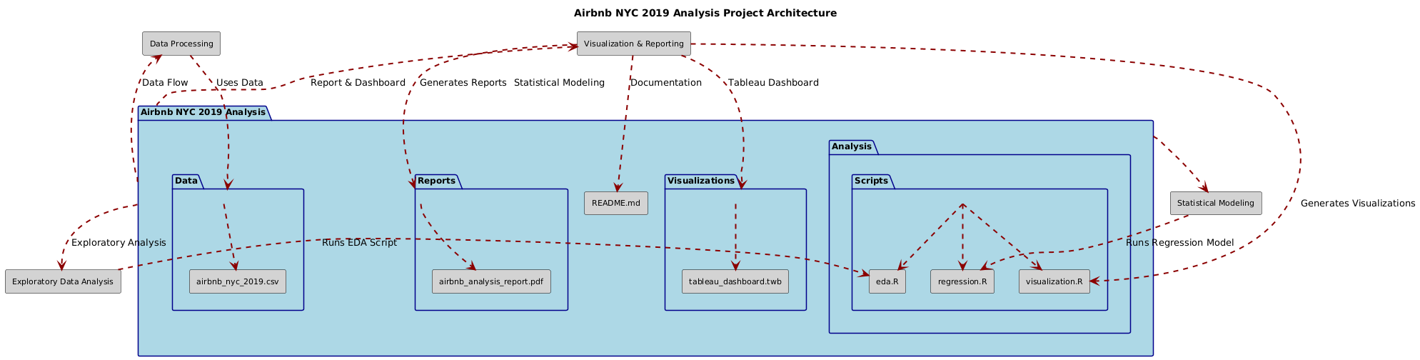
. ├── Data/ │ ├── airbnb_nyc_2019.csv ├── Analysis/ │ ├── scripts/ │ │ ├── eda.R │ │ ├── regression.R │ │ └── visualization.R ├── Visualizations/ │ ├── tableau_dashboard.twb ├── Reports/ │ ├── airbnb_analysis_report.pdf ├── README.md
The Airbnb Analysis Report includes:

Feel free to fork the repository and suggest improvements or enhancements. For questions or collaborations, please reach out via LinkedIn.
Author: Syed Faizan
Master’s Student in Data Analytics and Machine Learning
Northeastern University, Canada
| #---------------------------------------------------------# | |
| # Airbnb: Analysis of Short-Term Rentals by Syed Faizan # | |
| # # | |
| # # | |
| # # | |
| # # | |
| # # | |
| # # | |
| # # | |
| # # | |
| #---------------------------------------------------------# | |
| #Starting with a clean environment---- | |
| rm(list=ls()) | |
| # Clearing the Console | |
| cat("\014") # Clears the console | |
| # Clearing scientific notation | |
| options(scipen = 999) | |
| #Loading the packages utilized for Data cleaning and Data Analysis----- | |
| library(tidyverse) | |
| library(grid) | |
| library(gridExtra) | |
| library(dplyr) | |
| library(kableExtra) | |
| library(ggplot2) | |
| library(caret) | |
| library(rms) | |
| library(DataExplorer) | |
| library(dlookr) | |
| library(lubridate) | |
| library(MASS) | |
| library(pROC) | |
| library(dplyr) | |
| library(table1) | |
| # Loading the Data set | |
| abnb <- read.csv("airbnb_nyc.csv") | |
| # Overview of the Dataset | |
| summary(abnb) | |
| names(abnb) | |
| #View(abnb) | |
| abnb <- data.frame(abnb) | |
| # Checking for Missing values---- | |
| plot_missing(abnb) | |
| sum(is.na(abnb)) # 10,052 values missing from the column 'reviews_per_month'. None missing in other columns. | |
| # Decision to remove this column along with 'id', 'host_id', 'host_name', 'name' from the Dataset | |
| abnb <- abnb %>% | |
| dplyr::select( - id, - host_id, - host_name, - name, - reviews_per_month) | |
| # Descriptive statistics---- | |
| library(psych) | |
| psych::describe(abnb) %>% | |
| kable() | |
| library(vtable) | |
| st(abnb) | |
| table1(abnb, labels = (table)) | |
| ?table1() | |
| descriptive_table <- abnb %>% | |
| diagnose_numeric() | |
| descriptive_table | |
| # Basic Visualizations prior to Exploratory Data Analysis---- | |
| # Normality plots | |
| plot_normality(abnb) | |
| # Outlier Plot - Note that there are no outliers in 'availability' | |
| plot_outlier(abnb[ , c(6:8, 10:11)]) | |
| # Note that since 'price' is highly skewed we log transform it prior to visualization. | |
| # Plot of log transformed 'Price' by neighborhood | |
| abnb %>% | |
| ggplot(aes(price, fill = neighbourhood_group)) + | |
| geom_histogram(position = "identity", alpha = 0.5, bins = 20) + | |
| scale_x_log10(labels = scales::dollar_format()) + | |
| labs(fill = NULL, x = "price") | |
| # table of price by neighborhood | |
| price_by_neighborhood <- abnb %>% | |
| group_by(neighbourhood_group) %>% | |
| summarise(mean_price = mean(price)) | |
| kable(price_by_neighborhood) | |
| # Room type by neighborhood visualized | |
| ggplot(abnb, aes(neighbourhood_group)) + geom_bar(aes(fill = room_type)) + ggtitle("Room type by Neighborhood group") | |
| library(dplyr) | |
| # Count istings for each combination of neighbourhood_group and room_type | |
| roomtype_by_neighborhood <- abnb %>% | |
| group_by(neighbourhood_group, room_type) %>% | |
| summarise(total_listings = n(), .groups = 'drop') | |
| kable(roomtype_by_neighborhood) | |
| # mean price by room type and neighbourhood | |
| roomtype_by_neighborhood_meanprice <- abnb %>% | |
| group_by(neighbourhood_group, room_type) %>% | |
| summarise(mean_price = mean(price), .groups = 'drop') | |
| # map by mean price log transformed | |
| abnb %>% | |
| ggplot(aes(longitude, latitude, z = log(price))) + | |
| stat_summary_hex(alpha = 0.8, bins = 70) + | |
| scale_fill_viridis_c() + | |
| labs(fill = "Mean price (log)") | |
| # plot of price by neighborhood as different plots | |
| # Plot of log transformed 'Price' by neighborhood | |
| abnb %>% | |
| ggplot(aes(log(price))) + | |
| geom_histogram(aes(y = ..density..), bins = 30, fill = 'purple') + | |
| geom_density( alpha = 0.2, fill = 'purple') + | |
| scale_x_log10(labels = scales::dollar_format()) + | |
| facet_wrap(~ neighbourhood_group) + | |
| labs(fill = NULL, x = "Log price by neighborhood") | |
| # plot of above average price room types by neighbourood | |
| # Calculate the average price once, outside the filter | |
| average_price <- mean(abnb$price, na.rm = TRUE) | |
| abnb %>% | |
| filter(price >= average_price) %>% # Filter rows where price is above average | |
| group_by(neighbourhood_group, room_type) %>% | |
| tally() %>% | |
| ggplot(aes(x = reorder(neighbourhood_group, n), y = n, fill = room_type)) + # Reorder based on count 'n' | |
| geom_bar(stat = "identity") + # Specify bar chart | |
| labs(title = "Above Average Price by Neighborhood and Room Type", | |
| x = "Neighborhood Group", y = "Count of Listings", fill = "Room Type") | |
| # Box plots of log price by room type | |
| abnb %>% | |
| ggplot(aes(x = room_type, y = price)) + | |
| geom_boxplot(aes(fill = room_type)) + scale_y_log10() + | |
| ylab("Price") + | |
| xlab("Room Type") + | |
| ggtitle("Boxplots of Price by room type") + | |
| geom_hline(yintercept = mean(log(abnb$price)), linetype = 2, color = "purple") | |
| # Box plots of log price by neighborhood group | |
| abnb %>% | |
| ggplot(aes(x = neighbourhood_group, y = price)) + | |
| geom_boxplot(aes(fill = neighbourhood_group)) + scale_y_log10() + | |
| ylab("Price") + | |
| xlab("Neighborhood Group") + | |
| ggtitle("Boxplots of Price by Neighbourhood Group") + | |
| geom_hline(yintercept = mean(log(abnb$price)), linetype = 2, color = "purple") | |
| # Pair plots for the numeric variables | |
| # Create a new dataframe with only the numerical variables | |
| #Add log transformed price and retain only the numerical variables in the subset abnb_n | |
| abnb_n <- abnb %>% | |
| mutate(log_price = log1p(price)) | |
| abnb_n <- abnb_n %>% | |
| select_if(is.numeric) | |
| abnb_n <- abnb_n[ , c(4:8)] | |
| names(abnb_n) | |
| #Scatterplots of the numeric variables | |
| library(ggplot2) | |
| library(gridExtra) | |
| df <- abnb_n | |
| # Scatterplot of Log Transformed Price vs. Minimum Nights | |
| ggplot(data = df, aes(x = log_price, y = minimum_nights)) + | |
| geom_point(color = "red") + | |
| labs(title = "Log Transformed Price vs. Minimum Nights", x = "Log Transformed Price", y = "Minimum Nights") | |
| # Scatterplot of Log Transformed Price vs. Number of Reviews | |
| ggplot(data = df, aes(x = log_price, y = number_of_reviews)) + | |
| geom_point(color = "magenta") + | |
| labs(title = "Log Transformed Price vs. Number of Reviews", x = "Log Transformed Price", y = "Number of Reviews") | |
| # Scatterplot of Log Transformed Price vs. Calculated Host Listings Count | |
| ggplot(data = df, aes(x = log_price, y = calculated_host_listings_count)) + | |
| geom_point(color = "green") + | |
| labs(title = "Log Transformed Price vs. Host Listings Count", x = "Log Transformed Price", y = "Host Listings Count") | |
| # Scatterplot of Log Transformed Price vs. Availability 365 | |
| ggplot(data = df, aes(x = log_price, y = availability_365)) + | |
| geom_point(color = "pink") + | |
| labs(title = "Log Transformed Price vs. Availability 365", x = "Log Transformed Price", y = "availability_365") | |
| # Using the techniques practiced in ALY 6015 course as required by the assignment rubric | |
| # We perform Chi-Square and ANOVA tests between the suitable variables---- | |
| # Convert categorical variables to factors | |
| abnb$neighbourhood_group <- as.factor(abnb$neighbourhood_group) | |
| abnb$room_type <- as.factor(abnb$room_type) | |
| # Chi-Square Test of Independence between neighbourhood_group and room_type | |
| chi_test_result <- chisq.test(table(abnb$neighbourhood_group, abnb$room_type)) | |
| chi_test_result | |
| # Contingency table for chi-square test | |
| table1(~ room_type | neighbourhood_group, data=abnb, topclass="Rtable1-zebra", caption = "<b>Contengency Table for Chi-square test</b>") | |
| # ANOVA for Price by Neighbourhood Group | |
| anova_price_ng <- aov(price ~ neighbourhood_group, data = abnb) | |
| summary(anova_price_ng) | |
| TukeyHSD(anova_price_ng) | |
| # ANOVA for Price by Room Type | |
| anova_price_rt <- aov(price ~ room_type, data = abnb) | |
| summary(anova_price_rt) | |
| TukeyHSD(anova_price_rt) | |
| # ANOVA for Number of Reviews by Neighbourhood Group | |
| anova_reviews_ng <- aov(number_of_reviews ~ neighbourhood_group, data = abnb) | |
| summary(anova_reviews_ng) | |
| TukeyHSD(anova_reviews_ng) | |
| # Two way ANOVA for the interaction between Rooms and Neighbourhood | |
| anova_two_way <- aov(price ~ neighbourhood_group*room_type, data = abnb) | |
| summary(anova_two_way) | |
| TukeyHSD(anova_two_way) | |
| # correlation analysis | |
| # Confirming the numerical variables data frame | |
| names(abnb_n) | |
| library(ggcorrplot) | |
| cor_matrix <- cor(abnb_n) | |
| ggcorrplot(cor_matrix, lab = TRUE) | |
| # Linear regression model----- | |
| names(abnb_n) | |
| model_linear <- lm(log_price ~ . , data = abnb_n) | |
| summary(model_linear) | |
| plot(model_linear) | |
| # Looking for Outliers in the model | |
| library(car) | |
| outlierTest(model_linear) | |
| vif(model_linear) | |
| # Logisitic Model to predict price by room type---- | |
| # Load necessary libraries | |
| library(caret) | |
| library(pROC) | |
| library(dplyr) | |
| # Encoding room type into a binary categorical variable | |
| abnb$room_binary <- ifelse(abnb$room_type == "Entire home/apt", "home", "room") | |
| abnb$room_binary <- as.factor(abnb$room_binary) | |
| # Encoding price into a binary categorical variable | |
| threshold <- median(abnb$price) | |
| abnb$price_binary <- ifelse(abnb$price > threshold, "high", "low") | |
| abnb$price_binary <- as.factor(abnb$price_binary) | |
| abnb$price_binary <- relevel(abnb$price_binary, ref = "low") | |
| # Convert neighbourhood_group to factor | |
| abnb$neighbourhood_group <- as.factor(abnb$neighbourhood_group) | |
| # Set seed for reproducibility | |
| set.seed(123) | |
| # Splitting the data | |
| trainIndex <- createDataPartition(abnb$price_binary, p = 0.7, list = FALSE, times = 1) | |
| train_data <- abnb[trainIndex,] | |
| test_data <- abnb[-trainIndex,] | |
| # Fitting logistic regression model on training data | |
| logistic_model_train <- glm(price_binary ~ room_binary + minimum_nights + neighbourhood_group + availability_365, | |
| data = train_data, family = "binomial") | |
| summary(logistic_model_train) | |
| train_data %>% | |
| group_by(price_binary) %>% | |
| count() | |
| # Predicting on the train data | |
| predicted_probabilities_train <- predict(logistic_model_train, train_data, type = "response") | |
| predicted_classes_train <- ifelse(predicted_probabilities_train > 0.5, "high", "low") | |
| predicted_classes_train <- factor(predicted_classes_train, levels = c("low", "high")) | |
| # Generate the confusion matrix for training data | |
| conf_matrix_train <- confusionMatrix(predicted_classes_train, train_data$price_binary, positive = "high") | |
| print(conf_matrix_train) | |
| # Generating ROC curve for training data | |
| roc_object_train <- roc(response = train_data$price_binary, | |
| predictor = as.numeric(predicted_probabilities_train), | |
| levels = c("low", "high")) | |
| # Plotting ROC curve for training data | |
| plot(roc_object_train, main = "ROC Curve - Training Data", col = "#1c61b6") | |
| auc_value_train <- auc(roc_object_train) | |
| print(paste("Area Under the Curve (AUC) - Training Data:", auc_value_train)) | |
| text(x = 0.6, y = 0.2, labels = paste("AUC =", round(auc_value_train, 3)), col = "#ff0000", cex = 1.2) | |
| # Predicting on the test data | |
| predicted_probabilities_test <- predict(logistic_model_train, test_data, type = "response") | |
| predicted_classes_test <- ifelse(predicted_probabilities_test > 0.5, "high", "low") | |
| predicted_classes_test <- factor(predicted_classes_test, levels = c("low", "high")) | |
| # Generate the confusion matrix for test data | |
| conf_matrix_test <- confusionMatrix(predicted_classes_test, test_data$price_binary, positive = "high") | |
| print(conf_matrix_test) | |
| # Generating ROC curve for test data | |
| roc_object_test <- roc(response = test_data$price_binary, | |
| predictor = as.numeric(predicted_probabilities_test), | |
| levels = c("low", "high")) | |
| # Plotting ROC curve for test data | |
| plot(roc_object_test, main = "ROC Curve - Test Data", col = "#ff0000") | |
| auc_value_test <- auc(roc_object_test) | |
| print(paste("Area Under the Curve (AUC) - Test Data:", auc_value_test)) | |
| text(x = 0.6, y = 0.2, labels = paste("AUC =", round(auc_value_test, 3)), col = "#ff0000", cex = 1.2) | |
| # Plotting ROC curves for comparison | |
| plot(roc_object_train, main = "ROC Curve Comparison", col = "#1c61b6") | |
| text(x = 0.6, y = 0.4, labels = paste("AUC Train =", round(auc_value_train, 3)), col = "#1c61b6", cex = 1.2) | |
| lines(roc_object_test, col = "#ff0000") | |
| text(x = 0.6, y = 0.3, labels = paste("AUC Test =", round(auc_value_test, 3)), col = "#ff0000", cex = 1.2) | |
| legend("bottomright", legend = c("Train", "Test"), col = c("#1c61b6", "#ff0000"), lty = 1) | |
| library(knitr) | |
| # Create data frame | |
| comparison_data <- data.frame( | |
| Metric = c("Accuracy", "Kappa", "Sensitivity", "Specificity", "Positive Predictive Value", "Negative Predictive Value", "Prevalence", "Detection Rate", "Balanced Accuracy"), | |
| Training = c(0.8208, 0.6416, 0.8339, 0.8077, 0.8123, 0.8297, 0.4995, 0.4165, 0.8208), | |
| Testing = c(0.8199, 0.6399, 0.8310, 0.8089, 0.8127, 0.8275, 0.4995, 0.4151, 0.8199) | |
| ) | |
| # Generate the table using kable | |
| kable_table <- kable(comparison_data, | |
| col.names = c("Metric", "Training Data", "Testing Data"), | |
| caption = "Comparison of Metrics for Training and Testing Data", | |
| align = c('l', 'c', 'c')) # Use "latex" for LaTeX output, "html" for HTML | |
| # Display the table in the console or R Markdown | |
| print(kable_table) | |
| #Ridge and LASSO regression---- | |
| abnb$room_binary <- as.factor(abnb$room_binary) #Factorizing the room binary variable | |
| summary(abnb$room_binary) | |
| class(abnb$room_binary) #confirming factor | |
| abnb %>% | |
| group_by(room_type) %>% #confirming the counts of different rooms | |
| count() | |
| # giving back room binary character entries of 'home' and 'room' to avoid confusion | |
| abnb$room_binary <- as.factor(ifelse(abnb$room_type == "Entire home/apt", "home", "room")) | |
| abnb$neighbourhood_group <- as.factor(abnb$neighbourhood_group) | |
| unique(abnb$neighbourhood_group) | |
| relevel(abnb$neighbourhood_group, ref = "Staten Island") | |
| library(glmnet) | |
| class(abnb$room_binary) | |
| summary(abnb$room_binary) #checking in room binary is a factor | |
| range(abnbm$price) | |
| #creating a new subset for ridge and LASSO modelling | |
| names(abnb) | |
| abnbm <- abnb %>% | |
| select(neighbourhood_group,room_binary,number_of_reviews,price,minimum_nights, availability_365,calculated_host_listings_count) | |
| abnbm$neighbourhood_group <- as.factor(abnbm$neighbourhood_group) | |
| unique(abnbm$neighbourhood_group) | |
| relevel(abnbm$neighbourhood_group, ref = "Staten Island") | |
| levels(abnbm$neighbourhood_group) | |
| abnbm$room_binary <- as.factor(abnbm$room_binary) | |
| unique(abnbm$room_binary) | |
| relevel(abnbm$room_binary, ref = "room") | |
| trainIndex <- createDataPartition(abnbm$room_binary, p = 0.70, list = FALSE, times = 1) | |
| trainData <- abnbm[trainIndex, ] | |
| testData <- abnbm[-trainIndex, ] | |
| summary(trainData) | |
| relevel(trainData$neighbourhood_group, ref = "Staten Island") | |
| relevel(testData$neighbourhood_group, ref = "Staten Island") | |
| # Preparing the model matrix of predictors and the vector of the response variable | |
| train_x <- model.matrix(price ~ . -1, data = trainData) | |
| train_y <- trainData$price | |
| test_x <- model.matrix(price ~ . -1, data = testData) | |
| test_y <- testData$price | |
| # Ridge Regression | |
| set.seed(314) | |
| cv.ridge <- cv.glmnet(x = train_x, y = train_y, alpha = 0, standardize = TRUE) | |
| bestlam_ridge <- cv.ridge$lambda.min | |
| bestlam_1se_ridge <- cv.ridge$lambda.1se | |
| bestlam_ridge | |
| log(bestlam_ridge) | |
| bestlam_1se_ridge | |
| log(bestlam_1se_ridge) | |
| plot(cv.ridge) | |
| levels(abnbm$neighbourhood_group) | |
| ridge.mod <- glmnet(x = train_x, y = train_y, alpha = 0, lambda = bestlam_ridge) | |
| coef.ridge <- coef(ridge.mod) | |
| ridge.mod | |
| coef.ridge | |
| plot(glmnet(x = train_x, y = train_y, alpha = 0), xvar = "lambda", label = TRUE) | |
| abline(v = log(c(bestlam_ridge, bestlam_1se_ridge)), col = c("green", "purple")) | |
| plot(glmnet(x = train_x, y = train_y, alpha = 0), xvar = "dev", label = TRUE) | |
| abline(v = log(c(bestlam_ridge, bestlam_1se_ridge)), col = c("green", "purple")) | |
| preds_ridge_train <- predict(ridge.mod, newx = train_x) | |
| preds_ridge_test <- predict(ridge.mod, newx = test_x) | |
| rmse_train_ridge <- sqrt(mean((train_y - preds_ridge_train)^2)) | |
| rmse_test_ridge <- sqrt(mean((test_y - preds_ridge_test)^2)) | |
| rmse_test_ridge | |
| rmse_train_ridge | |
| # LASSO | |
| set.seed(324) | |
| cv.lasso <- cv.glmnet(x = train_x, y = train_y, alpha = 1) | |
| bestlam_lasso <- cv.lasso$lambda.min | |
| bestlam_1se_lasso <- cv.lasso$lambda.1se | |
| plot(cv.lasso) | |
| lasso.mod <- glmnet(x = train_x, y = train_y, alpha = 1, lambda = 2.71) | |
| coef.lasso <- coef(lasso.mod) | |
| coef.lasso | |
| plot(glmnet(x = train_x, y = train_y, alpha = 1), xvar = "lambda", label = TRUE) | |
| abline(v = log(c(bestlam_lasso, bestlam_1se_lasso)), col = c("blue", "red")) | |
| plot(glmnet(x = train_x, y = train_y, alpha = 1), xvar = "dev", label = TRUE) | |
| abline(v = log(c(bestlam_lasso, bestlam_1se_lasso)), col = c("blue", "red")) | |
| preds_lasso_train <- predict(lasso.mod, newx = train_x) | |
| preds_lasso_test <- predict(lasso.mod, newx = test_x) | |
| rmse_train_lasso <- sqrt(mean((train_y - preds_lasso_train)^2)) | |
| rmse_test_lasso <- sqrt(mean((test_y - preds_lasso_test)^2)) | |
| # Outputting RMSE results for comparison | |
| cat("Training RMSE Ridge: ", rmse_train_ridge, "") | |
| cat("Test RMSE Ridge: ", rmse_test_ridge, "") | |
| cat("Training RMSE LASSO: ", rmse_train_lasso, "") | |
| cat("Test RMSE LASSO: ", rmse_test_lasso, "") | |
| summary(abnbm$room_binary) | |
| coef(ridge.mod) | |
| summary(ridge.mod) | |
| coef(lasso.mod) | |
| library(knitr) | |
| # Constructing the data frame with RMSE results | |
| results_df <- data.frame( | |
| Model = c("Ridge", "LASSO"), | |
| Training_RMSE = c(rmse_train_ridge, rmse_train_lasso), | |
| Testing_RMSE = c(rmse_test_ridge, rmse_test_lasso) | |
| ) | |
| # Using kable to create a formatted table | |
| kable_table <- kable(results_df, | |
| col.names = c("Model", "Training RMSE", "Testing RMSE"), | |
| caption = "Comparison of RMSE Values for Ridge and LASSO Regression Models", | |
| align = c('l', 'c', 'c')) # Use "latex" for LaTeX output, "html" for HTML | |
| # To display the table in an R Markdown document or similar environment | |
| print(kable_table) | |
| # Appendix - additional tables with table1 package | |
| library(table1) | |
| names(abnb) | |
| render.median.IQR <- function(x, ...) { | |
| if (is.numeric(x)) { | |
| # Calculate statistics only if x is numeric | |
| c('', | |
| `Mean (SD)` = sprintf("%s (%s)", round(mean(x, na.rm = TRUE), 2), round(sd(x, na.rm = TRUE), 2)), | |
| `Median [IQR]` = sprintf("%s [%s, %s]", median(x, na.rm = TRUE), | |
| quantile(x, 0.25, na.rm = TRUE), quantile(x, 0.75, na.rm = TRUE))) | |
| } else { | |
| # Count frequencies of each category for non-numeric data | |
| levels_counts = table(x) | |
| counts = sapply(names(levels_counts), function(lvl) sprintf("%s: %d", lvl, levels_counts[lvl])) | |
| c('', `Counts` = paste(counts, collapse = ", ")) | |
| } | |
| } | |
| table1(~ neighbourhood_group + price + number_of_reviews + minimum_nights + availability_365 + calculated_host_listings_count|room_type , data=abnb, topclass="Rtable1-zebra") | |
| table1(~ + price + number_of_reviews + minimum_nights + availability_365 + calculated_host_listings_count + room_type| neighbourhood_group, data=abnb, topclass="Rtable1-zebra", render = render.median.IQR) |


© 2025 Syed Faizan. All Rights Reserved.