Loan Approval Prediction

💰 Loan Approval Prediction Using Machine Learning

MAIN TOOL

R Programming Language

Secondary tool

Tableau

INDUSTRY

Housing

📚 About the Project

This project focuses on predicting loan approval using a variety of machine learning models, including Logistic Regression, Decision Trees, Random Forests, and Gradient Boosting. The analysis is based on the Loan Dataset, comprising 614 records and 13 attributes related to loan applicants. The aim is to automate and optimize the loan approval process while maintaining high accuracy and consistency.

🔑 Key Features

Data Preprocessing:
- Addressed missing values using k-Nearest Neighbor (kNN) imputation.
- Feature transformations like scaling and log transformations for better model performance.
Modeling Techniques:
- Logistic Regression with feature selection.
- Advanced tree-based models like Random Forests and XGBoost.
- Support Vector Machines with SMOTE to handle class imbalance.
Evaluation Metrics:
- Accuracy, sensitivity, specificity, and ROC-AUC for model comparison.
- Confusion matrices and variable importance plots for interpretability.
Insights and Business Impact:
- Identified key predictors influencing loan approval, such as Credit History, Loan Amount, and Marital Status.
- Recommended ensemble methods for robust and scalable loan evaluation systems.

📊 Key Insights

Best Performing Model: Random Forest achieved the highest accuracy with a robust balance of sensitivity and specificity.
Critical Predictors:
- Credit History: The strongest determinant of loan approval.
- Loan Amount: Higher amounts are associated with reduced approval rates.
- Property Area: Urban and semiurban properties showed distinct approval patterns.
Model Comparison:
- Logistic Regression and Decision Trees provided interpretable results.
- Ensemble methods (Random Forest and XGBoost) demonstrated superior performance in accuracy and robustness.

📜 Full Report

For a detailed analysis, including methodology, visualizations, and results, refer to the complete project report:
📄 Loan Approval Prediction Report

📂 Project Structure

.
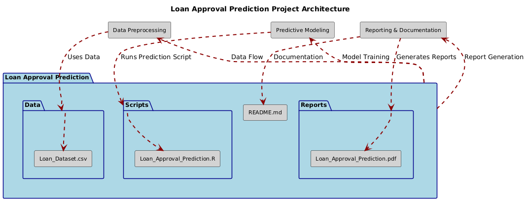
├── Data/
│   ├── Loan_Dataset.csv
├── Scripts/
│   ├── Loan_Approval_Prediction.R
├── Reports/
│   ├── Loan_Approval_Prediction.pdf
├── README.md

🤝 Connect with Me

Feel free to reach out for feedback, questions, or collaboration opportunities:
LinkedIn: Dr. Syed Faizan

Author: Syed Faizan
Master’s Student in Data Analytics and Machine Learning

Github Repository

R Code and the Report of the Analysis

	#---------------------------------------------------------#
	#Loan Approval Prediction - Syed Faizan #
	# #
	#---------------------------------------------------------#

	# Starting with a clean environment
	rm(list=ls())

	# Clearing the Console
	cat("\014") # Clears the console

	# Clearing scientific notation
	options(scipen = 999)

	# Loading the necessary packages for Data cleaning and Analysis

	# Installing libraries if not already installed


	# Loading libraries
	library(rpart, quietly = TRUE)
	library(caret, quietly = TRUE)
	library(randomForest, quietly = TRUE)
	library(ipred, quietly = TRUE)
	library(xgboost, quietly = TRUE)
	library(MASS, quietly = TRUE)
	library(rpart.plot, quietly = TRUE)
	library(rattle)
	library(readr)


	# Reading the data set as a data frame
	loanfinal <- read_csv("Loanfinal.csv")

	# Checking the structure of the data
	str(loanfinal)

	# Checking for missing values
	sum(is.na(loanfinal))

	library(DataExplorer)
	plot_missing(loanfinal)

	# Imputing missing values using KNN


	# Load the VIM library
	library(VIM)

	# Perform k-NN imputation
	loanfinal_imputed <- kNN(loanfinal, k = 5) # k = 5 is a commonly used default

	# Checking the structure after imputation
	str(loanfinal_imputed)

	# The kNN function adds additional columns with the suffix "_imp" to indicate
	# which values were imputed. If you want to remove these indicators:
	loanfinal_imputed <- loanfinal_imputed[, !grepl("_imp", names(loanfinal_imputed))]


	sum(is.na(loanfinal_imputed))

	loanfinal <- loanfinal_imputed
	# Dropping any unnecessary variables if applicable
	# e.g., loanfinal$some_column <- NULL

	# Analyzing the 'Loan_Status' variable
	table(loanfinal$Loan_Status)

	# Feature Engineering
	hist(loanfinal$ApplicantIncome,
	xlab = 'Applicant Income',
	ylab= 'Frequency',
	main = 'Histogram of Applicant Income',
	col = 'red')

	# Try square root transformation
	AppIncomesqrt <- sqrt(loanfinal$ApplicantIncome)
	hist(AppIncomesqrt,
	xlab = 'Square Root of Applicant Income',
	ylab= 'Frequency',
	main = 'Histogram of Applicant Income',
	col = 'blue')

	# Apply transformation


	loanfinal$ApplicantIncome <- sqrt(loanfinal$ApplicantIncome)

	#Apply similar transformations to other numeric variables after visualization

	# Coapplicant Income
	hist(loanfinal$CoapplicantIncome,
	xlab = 'Coapplicant Income',
	ylab = 'Frequency',
	main = 'Histogram of Coapplicant Income',
	col = 'green',
	breaks = 50)

	# Trying square root transformation
	CoappIncomesqrt <- sqrt(loanfinal$CoapplicantIncome)
	hist(CoappIncomesqrt,
	xlab = 'Square Root of Coapplicant Income',
	ylab = 'Frequency',
	main = 'Histogram of Square Root of Coapplicant Income',
	col = 'purple',
	breaks = 50)


	# Add a small constant to avoid log(0)
	CoappIncome_log <- log(loanfinal$CoapplicantIncome + 1)

	# Plot the histogram after log transformation
	hist(CoappIncome_log,
	xlab = 'Log of Coapplicant Income',
	ylab = 'Frequency',
	main = 'Histogram of Log Transformed Coapplicant Income',
	col = 'lightblue',
	breaks = 50)

	sum(loanfinal$CoapplicantIncome == 0) #There are 273 zeros in this column

	# I have decided to thus turn it into categorical column with 'yes' or 'no' as levels

	loanfinal$CoapplicantIncome <- ifelse(loanfinal$CoapplicantIncome != 0, 'yes', 'no')

	table(loanfinal$CoapplicantIncome) # 273 No and 341 Yes

	loanfinal$CoapplicantIncome <- factor(loanfinal$CoapplicantIncome, levels = c('yes','no')) #factorize co-applicant income

	# confirm factorization and the levels

	class(loanfinal$CoapplicantIncome)
	levels(loanfinal$CoapplicantIncome)

	# Convert all character columns to factors
	loanfinal[sapply(loanfinal, is.character)] <- lapply(loanfinal[sapply(loanfinal, is.character)], as.factor)


	str(loanfinal)

	# visualization

	library(ggplot2)

	ggplot(loanfinal, aes(x = CoapplicantIncome, fill = factor(Loan_Status))) +
	geom_histogram(color = "red", alpha = 0.7, stat="count", bins = 30) +
	scale_fill_manual(values = c("Y" = "blue", "N" = "orange")) + # Using actual levels from Loan_Status
	labs(x = "Coapplicant Income", fill = "Loan Status") +
	ggtitle("Coapplicant Income by Loan Status") +
	theme_bw()


	# LoanAmount
	hist(loanfinal$LoanAmount,
	xlab = 'Loan Amount',
	ylab = 'Frequency',
	main = 'Histogram of Loan Amount',
	col = 'orange',
	breaks = 50)

	# Try square root transformation
	LoanAmountsqrt <- sqrt(loanfinal$LoanAmount)
	hist(LoanAmountsqrt,
	xlab = 'Square Root of Loan Amount',
	ylab = 'Frequency',
	main = 'Histogram of Square Root of Loan Amount',
	col = 'cyan',
	breaks = 50)

	# Apply transformation


	loanfinal$LoanAmount <- sqrt(loanfinal$LoanAmount)


	# Loan_Amount_Term
	hist(loanfinal$Loan_Amount_Term,
	xlab = 'Loan Amount Term',
	ylab = 'Frequency',
	main = 'Histogram of Loan Amount Term',
	col = 'pink',
	breaks = 50)

	# Since distribution appears to be discrete no transformation is contemplated
	# Data splicing
	set.seed(12345)
	train <- sample(1:nrow(loanfinal), size = ceiling(0.80 * nrow(loanfinal)), replace = FALSE)
	loan_train <- loanfinal[train, ]
	loan_test <- loanfinal[-train, ]

	loan_test$Loan_Status <- factor(loan_test$Loan_Status, levels = c('Y', 'N')) #confirming the levels in target variable
	loan_train$Loan_Status <- factor(loan_train$Loan_Status, levels = c('Y', 'N'))


	# Confirming the structure of the train data frame

	# Classification modelling
	# Logistic regression
	# Fit logistic regression model using all variables as predictors and Loan_Status as the response
	glm.fits <- glm(Loan_Status ~ Gender + Married + Dependents + Education + Self_Employed + ApplicantIncome +
	CoapplicantIncome + LoanAmount + Loan_Amount_Term + Credit_History + Property_Area,
	data = loan_train,
	family = binomial)

	# Summary of the model
	summary(glm.fits)

	# Coefficients of the model
	coef(glm.fits)

	# p-values of the coefficients
	summary(glm.fits)$coef[, 4]



	# Visual confirmation of loan status by Marital Status

	ggplot(loan_train, aes(x = Married, fill = factor(Loan_Status))) +
	geom_histogram(color = "red", alpha = 0.7, stat="count", bins = 30) +
	scale_fill_manual(values = c("Y" = "blue", "N" = "orange")) + # Using actual levels from Loan_Status
	labs(x = "Married", fill = "Loan Status") +
	ggtitle("Marital Status by Loan Status") +
	theme_bw()

	table(loan_train$Married, loan_train$Loan_Status) # [102, 62,
	# 238, 90]

	# I retrain the model using only the significant variables
	# Checking model fit on training data

	glm.fits_significant <- glm(Loan_Status ~ Married + Credit_History + Property_Area,
	data = loan_train,
	family = binomial)

	# Summary of the updated model
	summary(glm.fits_significant)

	# Predict probabilities for the model with significant variables
	glm.probs_significant <- predict(glm.fits_significant, type = "response")

	# Convert probabilities to class predictions (using 0.5 threshold)
	glm.pred_significant <- ifelse(glm.probs_significant > 0.5, "Y", "N")

	# Convert predictions and actual Loan_Status to factors
	glm.pred_significant <- factor(glm.pred_significant, levels = c("Y", "N"))
	loan_train$Loan_Status <- factor(loan_train$Loan_Status, levels = c("Y", "N"))

	# Confusion matrix using caret package for the model with significant variables
	conf_matrix_significant <- confusionMatrix(glm.pred_significant, loan_train$Loan_Status)

	# Print confusion matrix and performance metrics
	print(conf_matrix_significant)

	# Test data model fitting
	# Predict probabilities on the test set using the model with significant variables
	glm.probs_significant_test <- predict(glm.fits_significant, newdata = loan_test, type = "response")

	# Convert probabilities to class predictions (using 0.5 threshold) on the test set
	glm.pred_significant_test <- ifelse(glm.probs_significant_test > 0.5, "Y", "N")

	# Convert predictions and actual Loan_Status to factors for comparison
	glm.pred_significant_test <- factor(glm.pred_significant_test, levels = c("Y", "N"))
	loan_test$Loan_Status <- factor(loan_test$Loan_Status, levels = c("Y", "N"))

	# Confusion matrix using caret package for the test data
	conf_matrix_significant_test <- confusionMatrix(glm.pred_significant_test, loan_test$Loan_Status)

	# Print confusion matrix and performance metrics for the test set
	print(conf_matrix_significant_test)

	# ROC Curve

	# Load necessary libraries
	library(pROC) # For AUC and ROC calculations
	library(ggplot2) # For plotting

	# Predict probabilities on the test set using the model with significant variables
	glm.probs_significant_test <- predict(glm.fits_significant, newdata = loan_test, type = "response")

	# Create ROC object
	roc_obj <- roc(loan_test$Loan_Status, glm.probs_significant_test, levels = c("Y", "N"))

	# Print AUC value
	auc_value <- auc(roc_obj)
	print(paste("AUC:", auc_value))

	# Plot the ROC curve
	ggroc(roc_obj) +
	ggtitle(paste("ROC Curve (AUC =", round(auc_value, 2), ")")) +
	theme_bw()


	# Linear Discriminant Analysis

	# Load necessary packages
	library(MASS) # For LDA
	library(caret) # For confusionMatrix

	# In LDA and QDA only numerical variables can be used as a common covariance is assumed by LDA.
	# Extracting numeric columns from loan_train
	numeric_cols_train <- sapply(loan_train, is.numeric)
	train_numeric <- loan_train[, numeric_cols_train]
	# Extracting numeric columns from loan_test
	numeric_cols_test <- sapply(loan_test, is.numeric)
	test_numeric <- loan_test[, numeric_cols_test]
	# Checking the structure of the extracted numeric columns
	str(train_numeric)
	str(test_numeric)
	# Add Loan_Status to the numeric data
	train_numeric$Loan_Status <- loan_train$Loan_Status
	test_numeric$Loan_Status <- loan_test$Loan_Status

	# Now, fit the LDA model on training data using the numeric columns
	lda_model <- lda(Loan_Status ~ ., data = train_numeric)

	summary(lda_model)

	# Predict on the test data using numeric columns
	pred_lda <- predict(lda_model, test_numeric)$class

	# Create a confusion matrix (predictions first, actuals second)
	conf_matrix_lda <- confusionMatrix(pred_lda, test_numeric$Loan_Status)

	# Print the confusion matrix and performance metrics for LDA
	print(conf_matrix_lda)

	# Quadratic discriminant Analysis

	# Load necessary packages
	library(MASS) # For QDA
	library(caret) # For confusionMatrix

	# Fit QDA model on training data using numeric columns
	qda_model <- qda(Loan_Status ~ ., data = train_numeric)

	summary(qda_model)

	# Predict on the test data using numeric columns
	pred_qda <- predict(qda_model, test_numeric)$class

	# Create a confusion matrix (predictions first, actual observations second)
	conf_matrix_qda <- confusionMatrix(pred_qda, test_numeric$Loan_Status)

	# Print the confusion matrix and performance metrics for QDA
	print(conf_matrix_qda)

	# Tree Based modelling

	# Classification Tree ( model using rpart)
	tree <- rpart(Loan_Status ~ ., data = loan_train, method = "class")
	rpart.plot(tree, nn = TRUE)

	print(tree)
	summary(tree)

	# Best Complexity Parameter (Pruning the tree)
	cp.optim <- tree$cptable[which.min(tree$cptable[,"xerror"]),"CP"]
	tree.pruned <- prune(tree, cp = cp.optim)

	rpart.plot(tree.pruned, nn = TRUE)

	summary(tree.pruned)

	print(tree.pruned)

	# Testing the model with Pruned Tree
	pred_tree <- predict(object = tree.pruned, loan_test, type = "class")
	conf_matrix_tree <- confusionMatrix(table(loan_test$Loan_Status, pred_tree))

	print(conf_matrix_tree)


	# Bagging and Random Forests
	library(randomForest)

	ncol_train <- ncol(loan_train) - 1
	print(ncol_train) # 11 variables excepting the target variable Loan_Status.

	# Bagging: Random Forest with mtry = total number of predictors
	set.seed(1987)
	bag.loan <- randomForest(Loan_Status ~ ., data = loan_train, mtry = 11, importance = TRUE)

	# Print the bagging model details
	print(bag.loan)
	varImpPlot(bag.loan, main = "Variable Importance plot of bagging Tree model")
	summary(bag.loan)

	# Predict on the test set using Bagging model
	bag_pred <- predict(bag.loan, newdata = loan_test)

	# Confusion matrix for Bagging model predictions
	conf_matrix_bag <- confusionMatrix(bag_pred, loan_test$Loan_Status)
	print(conf_matrix_bag)

	# Random Forest: Random Forest with mtry = subset of predictors (p/3 is default but
	# shall use approximation of sqrt(p) that is near sqrt(11) which is 4)
	set.seed(314)
	rf.loan <- randomForest(Loan_Status ~ ., data = loan_train, mtry = 4, importance = TRUE)

	# Print the random forest model details
	print(rf.loan)
	varImpPlot(rf.loan, main = "Variable Importance plot of Random Tree model")
	summary(rf.loan)

	# Predict on the test set using Random Forest model
	rf_pred <- predict(rf.loan, newdata = loan_test)

	# Confusion matrix for Random Forest model predictions
	conf_matrix_rf <- confusionMatrix(rf_pred, loan_test$Loan_Status)
	print(conf_matrix_rf)

	# Boosting
	# Load necessary libraries
	# Load necessary libraries
	install.packages("xgboost")
	install.packages("caret")
	library(xgboost)
	library(caret)

	# Create new data sets loan_train1 and loan_test1 to avoid overwriting original data sets
	loan_train1 <- loan_train
	loan_test1 <- loan_test

	# Convert Loan_Status to a numeric binary (0 = N, 1 = Y) in the new data sets
	loan_train1$Loan_Status <- ifelse(loan_train1$Loan_Status == "Y", 1, 0)
	loan_test1$Loan_Status <- ifelse(loan_test1$Loan_Status == "Y", 1, 0)

	# Convert categorical variables to dummy variables using model.matrix()
	# Remove the intercept column generated by model.matrix() with `[, -1]`
	train_matrix <- model.matrix(Loan_Status ~ . - 1, data = loan_train1)
	test_matrix <- model.matrix(Loan_Status ~ . - 1, data = loan_test1)

	# Check the resulting train_matrix and test_matrix
	str(train_matrix)
	str(test_matrix)

	# Convert data to D Matrix format for xgboost
	dtrain <- xgb.DMatrix(data = train_matrix, label = train_label)
	dtest <- xgb.DMatrix(data = test_matrix, label = test_label)

	# Set parameters for xgboost (for binary classification)
	params <- list(
	objective = "binary:logistic", # For binary classification
	eval_metric = "error", # Use classification error as the evaluation metric
	max_depth = 4, # Maximum depth of trees
	eta = 0.1, # Learning rate (shrinkage)
	nthread = 2 # Number of threads for parallel computing
	)

	# Train the xgboost model
	set.seed(234)
	xgb_model <- xgboost(
	data = dtrain,
	params = params, # Parameters are provided here
	nrounds = 100, # Number of boosting rounds (trees)
	verbose = 0 # Turn off printing of boosting iterations
	)
	summary(xgb_model)
	# Predict on the test data
	xgb_pred_prob <- predict(xgb_model, dtest)
	# Convert predicted probabilities to binary class predictions using 0.5 as threshold
	xgb_pred <- ifelse(xgb_pred_prob > 0.5, 1, 0)
	# Confusion matrix using caret package (reconverting numeric predictions back to factors for evaluation)
	xgb_pred_factor <- factor(xgb_pred, levels = c(0, 1), labels = c("Y", "N"))
	test_label_factor <- factor(test_label, levels = c(0, 1), labels = c("Y", "N"))

	# Print confusion matrix and performance metrics
	conf_matrix_xgb <- confusionMatrix(xgb_pred_factor, test_label_factor)
	print(conf_matrix_xgb)

	# Advanced EDA using PCA and Clustering
	# Creating a Data frame with only numerical variables
	# Identify the numeric columns in the loan final data frame
	numeric_cols_final <- sapply(loanfinal, is.numeric)

	# Extract only the numeric columns into a new data frame
	final_numeric <- loanfinal[, numeric_cols_final]

	# View the first few rows of the numeric data frame
	head(final_numeric)

	# Implementing a Principal Component Analysis Model
	names(final_numeric)
	apply(final_numeric, 2, mean)
	apply(final_numeric, 2, var)
	pr.out=prcomp(final_numeric, scale=TRUE)
	names(pr.out)
	print(pr.out)
	summary(pr.out)
	par(mfrow = c(1, 1))

	plot(summary(pr.out)$importance[3,], ylab = "Cumulative Proportion of Variance Explained",
	xlab = "PC1 PC2 PC3 ", col= "red",pch= c(21, 22, 23, 24), cex = c(1,2,3,3), type = "b", bg = "yellow")
	title(main = "Cumulative Proportion of Variance Explained by the 3 Principal Components")

	pr.out$rotation=-pr.out$rotation
	pr.out$x=-pr.out$x
	biplot(pr.out, scale=0)

	pr.out$sdev
	pr.var=pr.out$sdev^2
	pr.var
	pve=pr.var/sum(pr.var)
	pve
	par(mfrow = c(1, 2))
	plot(pve, xlab="Principal Component", ylab="Proportion of Variance Explained", ylim=c(0,1), col= "purple",pch= c(21, 22, 23, 24), cex = c(1,2,3,3), type = "b", bg = "orange")
	plot(cumsum(pve), xlab="Principal Component", ylab="Cumulative Proportion of Variance Explained", ylim=c(0,1),col= "red",pch= c(21, 22, 23, 24), cex = c(1,2,3,3), type = "b", bg = "blue")

	# Hierarchical Clustering

	# Checking Correlation
	cor_matrix <- cor(final_numeric)

	library(ggcorrplot)
	ggcorrplot(cor_matrix, lab = TRUE)

	# Hierarchical clustering on different linkage methods
	hc.complete <- hclust(dist(final_numeric), method = "complete")
	hc.average <- hclust(dist(final_numeric), method = "average")
	hc.single <- hclust(dist(final_numeric), method = "single")

	# Set up a plotting area with 3 columns for subplots
	par(mfrow = c(1, 3))

	# Plot the dendrograms for different linkage methods
	plot(hc.complete, main = "Complete Linkage", xlab = "", sub = "", cex = .9)
	plot(hc.average, main = "Average Linkage", xlab = "", sub = "", cex = .9)
	plot(hc.single, main = "Single Linkage", xlab = "", sub = "", cex = .9)



	# Combining Hierarchical Clustering with PCA

	hc.out <- hclust(dist(pr.out$x[, 1:3]))
	plot(hc.out, main = "Hierarchical Clustering on Three Principal Components", xlab = "Observations")
	clusters <- cutree(hc.out,2 )
	table(clusters, loanfinal$Loan_Status) # clusters N Y 1 188 412
	# 2 4 10

	#SVM
	# Load necessary libraries
	library(e1071)
	library(ROCR)
	library(caret)
	library(caTools)


	library(smotefamily)


	# Apply SMOTE to balance the training data
	set.seed(123) # For reproducibility
	train_numeric_smote <- SMOTE(train_numeric[, -ncol(train_numeric)], # Exclude the target variable for SMOTE
	train_numeric$Loan_Status, # Target variable
	K = 5)

	# The SMOTE function from smotefamily package returns a list with 'data' that includes both features and the class
	train_smote <- train_numeric_smote$data

	# Ensure Loan_Status is a factor in the new dataset
	train_smote$Loan_Status <- as.factor(train_smote$class)

	# Drop the extra 'class' column (which is just a copy of Loan_Status)
	train_smote$class <- NULL

	# Check class distribution after SMOTE
	table(train_smote$Loan_Status)

	# Train an SVM model using the SMOTE-balanced data
	svmfit_smote <- svm(Loan_Status ~ ., data = train_smote, kernel = "radial", cost = 100, gamma = 4)
	summary(svmfit_smote)

	tune.smote.svm <- tune(svm, Loan_Status ~ ., data = train_smote, kernel = "radial",
	ranges = list(cost = c(0.1, 1, 10, 100, 1000),
	gamma = c(0.5, 1, 2, 3, 4)))
	summary(tune.smote.svm)

	# Tuned SVM modelwith best parameters
	svmfit_smote <- tune.smote.svm$best.model # since accuracy is low this may be due to overfitting
	# I shall try hyper parameter tuning


	# Ensure that Loan_Status in test_numeric is a factor
	test_numeric$Loan_Status <- as.factor(test_numeric$Loan_Status)

	# Use the trained SVM model (svmfit_smote) to make predictions on the test set
	ypred_test <- predict(svmfit_smote, test_numeric)

	# Create a confusion matrix to evaluate the predictions
	confusion_matrix_test <- table(Predicted = ypred_test, Actual = test_numeric$Loan_Status)
	print(confusion_matrix_test)

	# If you want to compute other metrics like accuracy, precision, recall, etc., you can use the caret package
	library(caret)

	# Compute confusion matrix and other performance metrics
	conf_matrix_svm <- confusionMatrix(ypred_test, test_numeric$Loan_Status)

	# Print the confusion matrix and performance metrics
	print(conf_matrix_svm)

	# Visualizing SVM on PCA


	# Load necessary libraries
	library(e1071)
	library(ggplot2)
	library(caret) # For evaluation metrics like confusion matrix

	# Step 1: Apply PCA on the training data (excluding the target variable)
	pca_model <- prcomp(train_smote[, -ncol(train_smote)], center = TRUE, scale. = TRUE)

	# Extract the first two principal components from the training data
	train_pca <- data.frame(PC1 = pca_model$x[, 1], PC2 = pca_model$x[, 2], Loan_Status = train_smote$Loan_Status)

	# Step 2: Tune SVM model on the PCA-transformed training data
	set.seed(123) # For reproducibility
	tune.out <- tune(svm, Loan_Status ~ ., data = train_pca, kernel = "radial",
	ranges = list(cost = c(0.1, 1, 10, 100),
	gamma = c(0.01, 0.1, 0.5, 1)))

	# Get the best model from the tuning process
	best_model <- tune.out$best.model

	# Step 3: Apply PCA on the test set (transform test data using the same PCA model)
	test_pca <- data.frame(PC1 = predict(pca_model, test_numeric[, -ncol(test_numeric)])[, 1],
	PC2 = predict(pca_model, test_numeric[, -ncol(test_numeric)])[, 2],
	Loan_Status = test_numeric$Loan_Status)

	# Step 4: Test the best model on the PCA-transformed test data
	pred_test <- predict(best_model, test_pca)

	# Confusion matrix to evaluate performance on the test set
	confusion_matrix_test <- confusionMatrix(pred_test, test_pca$Loan_Status)
	print(confusion_matrix_test)

	# Step 5: Plot the decision boundary using the best model

	# Create a grid of points for decision boundary visualization
	x_min <- min(train_pca$PC1) - 1
	x_max <- max(train_pca$PC1) + 1
	y_min <- min(train_pca$PC2) - 1
	y_max <- max(train_pca$PC2) + 1

	# Create a grid of values
	grid <- expand.grid(PC1 = seq(x_min, x_max, length.out = 200),
	PC2 = seq(y_min, y_max, length.out = 200))

	# Predict on the grid using the best model
	grid$Loan_Status <- predict(best_model, grid)
	grid$Loan_Status <- as.numeric(grid$Loan_Status) # Convert factor to numeric

	# Step 6: Plot the decision boundary
	ggplot() +
	geom_point(data = train_pca, aes(x = PC1, y = PC2, color = Loan_Status), size = 2) +
	geom_tile(data = grid, aes(x = PC1, y = PC2, fill = Loan_Status), alpha = 0.3) + # Better visualization
	labs(title = "SVM Decision Boundary on PCA-Transformed Data",
	x = "Principal Component 1",
	y = "Principal Component 2") +
	theme_minimal() +
	scale_color_manual(values = c("blue", "red")) +
	scale_fill_gradient(low = "lightblue", high = "yellow")

	# Print out the best parameters found during tuning
	print(tune.out$best.parameters)

	# Comparison of all the models
	# Create a function to extract metrics from a confusion matrix
	extract_metrics <- function(conf_matrix) {
	accuracy <- conf_matrix$overall['Accuracy']
	sensitivity <- conf_matrix$byClass['Sensitivity']
	specificity <- conf_matrix$byClass['Specificity']
	positive_predictive_value <- conf_matrix$byClass['Pos Pred Value'] # Precision

	return(c(accuracy, sensitivity, specificity, positive_predictive_value))
	}

	# Extracting metrics for each model
	metrics_logistic <- extract_metrics(conf_matrix_significant_test)
	metrics_lda <- extract_metrics(conf_matrix_lda)
	metrics_qda <- extract_metrics(conf_matrix_qda)
	metrics_tree <- extract_metrics(conf_matrix_tree)
	metrics_bagging <- extract_metrics(conf_matrix_bag)
	metrics_rf <- extract_metrics(conf_matrix_rf)
	metrics_xgb <- extract_metrics(conf_matrix_xgb)
	metrics_svm <- extract_metrics(conf_matrix_svm)
	# Combine all metrics into a data frame
	model_comparison <- data.frame(
	Model = c("Logistic Regression", "LDA", "QDA", "Decision Tree", "Bagging", "Random Forest", "XGBoost", "SVM"),
	Accuracy = c(metrics_logistic[1], metrics_lda[1], metrics_qda[1], metrics_tree[1], metrics_bagging[1], metrics_rf[1], metrics_xgb[1],metrics_svm[1] ),
	Sensitivity = c(metrics_logistic[2], metrics_lda[2], metrics_qda[2], metrics_tree[2], metrics_bagging[2], metrics_rf[2], metrics_xgb[2], metrics_svm[2]),
	Specificity = c(metrics_logistic[3], metrics_lda[3], metrics_qda[3], metrics_tree[3], metrics_bagging[3], metrics_rf[3], metrics_xgb[3], metrics_svm[3]),
	Positive_Predictive_Value = c(metrics_logistic[4], metrics_lda[4], metrics_qda[4], metrics_tree[4], metrics_bagging[4], metrics_rf[4], metrics_xgb[4], metrics_svm[4])
	)
	# Rank models by Accuracy
	model_comparison <- model_comparison[order(-model_comparison$Accuracy), ]

	# Display the results
	print(model_comparison)
	# This completes the Project

view raw LoanApproval.R hosted with ❤ by GitHub